+44(0)28 9032 2228
 Excel - Intro 2010/2013/365
 SQL Query Language Intro
 Power BI - Level 1 (1 - Day)
.jpg) Power Query
Power Query

-
 3/3/2025
CITB - The Construction Industry Training Board have included Mullan Training on their Approved List We deliver Trainings in Belfast Northern Ireland OR On Customer's Own Premises -
 30/4/2025
Microsoft Visio Training from Belfast Northern Ireland - Maximise the potential of the Visio application -
 3/3/2025
Intro to Microsoft PowerPoint Training from Belfast Northern Ireland - Online Training Course -
 3/3/2025
Microsoft 365 Training Courses now available inc Belfast, Omagh, Derry, Newry and Throughout Northern Ireland -
 6/5/2025
Intro to Crystal Reports Training from Belfast Northern Ireland - Virtual, Online - Learn how to create powerful and dynamic reports, presenting your data in an attractive format -
 3/3/2025
IT/Computer Room Hire in Belfast City Centre (Opposite Europa Hotel) - Call now to book -
 3/3/2025
Hot Course - 2 Day Advanced Microsoft Excel Course Training - CALL NOW TO BOOK -
 31/3/2025
Microsoft 365 training courses in Word, Excel, Access, Outlook, Powerpoint, Sharepoint in Belfast and Omagh Northern Ireland -
 14/4/2025
CLASSROOM & ONLINE Power BI Level 1 course -
3/3/2025
HOT COURSE - Intro to Microsoft Visio Training in Belfast Northern Ireland OR Virtually - CALL NOW to secure a place on this course -
 14/4/2025
New Course - Microsoft Power BI Introduction training from Belfast Northern Ireland - Classroom & Online Training -
 17/4/2025
HOT COURSE - Introduction to Microsoft Excel Training in Belfast Northern Ireland OR On your Own Premises - Call NOW to Book -
 3/3/2025
Need to Produce and Deliver Professional Presentations? Book NOW on our Advanced Microsoft PowerPoint course Training in Belfast Northern Ireland OR On your Own Premises - Limited places available -
 26/3/2025
Microsoft Sharepoint Introduction Training Course in Belfast NI -
 3/3/2025
Power BI Paginated Report Builder -
 3/3/2025
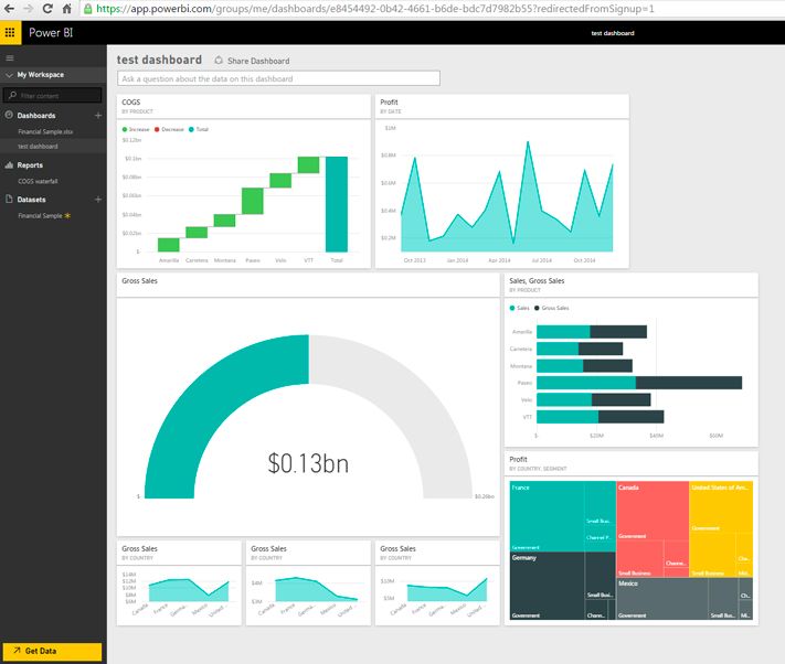
Data Visualisation & Presentation Techniques with Mullan IT Training -
 25/3/2025
Introduction to Microsoft Project Training from Belfast Northern Ireland - Classroom Based Training & Via Our Online Classrooms -
 20/3/2025
1 day Adv Microsoft Excel CourseTraining in Belfast Northern Ireland OR On your Own Premises - Places Available - Call Now to Book
Tips & Tricks
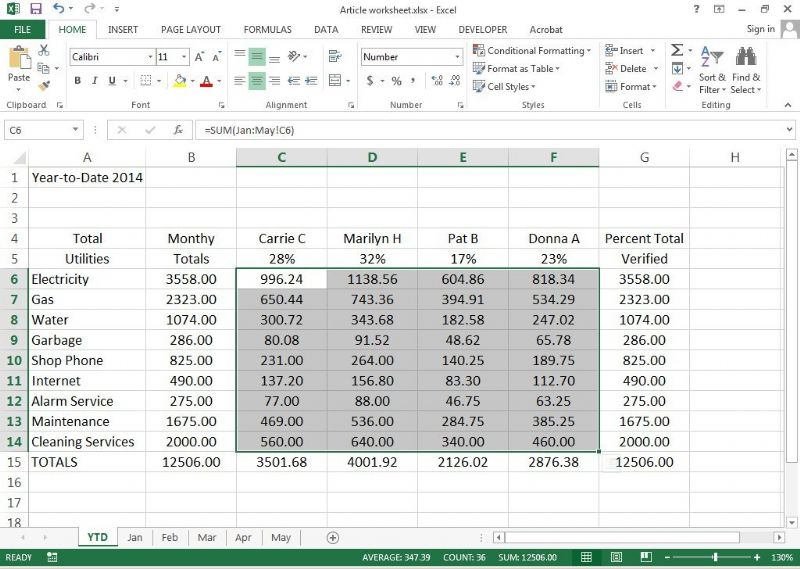
Weighted Averages in a PivotTable

A good example of how to use calculated fields is for summarizing data differently than you can normally summarize it with a PivotTable. When you create a PivotTable, you can use several different functions to summarize the data that is displayed. For instance, you can create an average of data in a particular field. What if you want to create a weighted average, however? Excel doesn't provide a function that automatically allows you to do this.
When you have special needs for summations - like weighted averages - the easiest way to achieve your goal is to add an additional column in the source data as an intermediate calculation, and then add a calculated field to the actual PivotTable.
For example, you could add a "Weighted Value" column to your source data. The formula in the column should multiply the weight times the value to be weighted. This means that if your weight is in column C and your value to be weighted is in column D, your formula in the Weighted Value column would simply be like =C2*D2. This formula will be copied down the entire column for all the rows of the data.
You are now ready to create your PivotTable, which you should do as normal with one exception: you need to create a Calculated Field. Follow these steps:
1. Click the down arrow next to the word PivotTable at the left side of the PivotTable toolbar. Excel displays a menu.
2. Choose Formulas | Calculated Fields. Excel displays the Insert Calculated Field dialog box. (See Figure 1.)
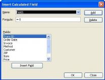
3. In the Name box, enter a name for your new field.
4. In the Formula box, enter the formula you want to be used for your weighted average, such as =Weighted Value/Weight. (You use field names in the formula; you can select them from the field list at the bottom of the Insert Calculated Field dialog box.)
5. Click OK.
Your calculated field is now inserted, and you can use the regular summation functions to display a sum of the calculated field; this is your weighted average.
Since there are many different ways that weighted averages can be calculated, it should go without saying that you can modify the formulas and steps presented here to reflect exactly what you need to be done with your data.
Formatting a PivotTable
You know that you can format cells in your worksheets by using the different tools on the Formatting toolbar, or by using the Cell option from the Format menu. Excel also allows you to format PivotTables using these same techniques. You should know, however, that the best way to format PivotTables is to use the AutoFormat feature. This is because whenever you manipulate the table or refresh the data, any explicit formatting you might have applied (using the Cell option from the Format menu) is eliminated by Excel. This limitation does not apply when you use the built-in AutoFormats.
To use the AutoFormat feature, select a cell in the PivotTable, and then choose AutoFormat from the Format menu. Excel displays the AutoFormat dialog box. (See Figure 1.)
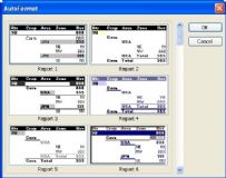
Figure 1. The AutoFormat dialog box.
Scroll through the available formats, and click the one you want to use. When you click the OK button, the desired format is applied to the PivotTable.
Maintaining Formatting when Refreshing PivotTables
PivotTables provide a great way to analyze large amounts of data and pull out the summarizations that you need. Once you have the PivotTable displaying the values you need, you can then format the table to make the data presentable - for a while. You see, when you update the data on which the PivotTable is based and then refresh the PivotTable, all your formatting work may go away.
The way around this is to follow these steps:
- Make sure that your PivotTable displays the values you want.
- Format the PivotTable in whatever way desired.
- On the PivotTable toolbar, choose Table Options from the PivotTable menu. Excel displays the PivotTable Options dialog box. (See Figure 1.)
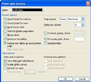
Figure 1. The PivotTable Options dialog box.
- Make sure the Preserve Formatting check box is selected.
- Click OK.
Now, when you refresh the PivotTable, your previously applied formatting should remain on rows and columns previously in the PivotTable. If the refresh results in new rows being added to the PivotTable, then you will still need to format those, unless you are using an AutoFormat.
Adding Vertical Lines at the Sides of a Word

Word allows you to easily add all sorts of flourishes to the text in your document. If you want to add vertical lines at the left and right of a word (perhaps for a page title), you can do so easily using any one of several different methods.
One way is to use the "pipe" character before and after your word. On most keyboards the pipe, or vertical bar, is a shifted version of the \ character. Type the pipe, a few spaces, the word, the same number of spaces, and then another pipe character. You can then center the paragraph.
If you are comfortable with the use of fields in a document, you could also try using the pipe character with the EQ field. Just insert a set of field braces (by pressing Ctrl+F9) and then making sure the field looks like this:
{eq \b \bc\| ( myword )}
When you collapse the field you end up with "myword" centered between the pipe characters.
Another method is to simply type your word and then format the paragraph so that it has borders at the left and right sides. Follow these steps:
- Make sure the insertion point is within the word for which there should be vertical lines on both sides.
- Display the Home tab of the ribbon.
- Click the down-arrow next to the Borders tool in the Paragraph group and then choose Borders and Shading. Word displays the Borders and Shading dialog box. (See Figure 1.)
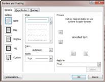
Figure 1. The Borders and Shading dialog box.
- Make sure the Borders tab is selected.
- Use the controls in the dialog box to add the desired border to both the left and right sides of the paragraph.
- Click on OK.
At this point you should see the borders on both sides of the paragraph. However, they are probably too far from the text, as the paragraph extends all the way from the left margin to the right. (This means that the borders appear at the left and right margins.) Adjust the left and right indents of the paragraph so that the vertical lines move in closer to the center. You can also adjust the other settings for the paragraph formatting (like Space Before and Space After) to get the paragraph exactly where you want it.
You can select the word itself and raise it or lower it in relation to the bordering lines in this manner:
- Select the word you want to adjust.
- Press Ctrl+D to display the Font dialog box.
- Make sure the Character Spacing tab (Word 2007) or Advanced tab (Word 2010) is selected. (See Figure 2.)
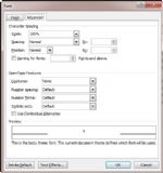
Figure 2. The Advanced tab of the Font dialog box.
- Using the Position drop-down list, choose either Raised or Lowered, as desired.
- Using the By box (to the right of the Position drop-down list) specify how far, in points, the text should be raised or lowered.
- Click OK.
Using the paragraph borders in this manner can require a lot of trial and error to get everything just right. If you use a table instead of a regular paragraph, the positioning is just a bit easier. Simply create a centered single-cell-table and make sure the cell is wide enough to contain the word you want. When you center the word in the table cell, you can then add borders to the left and right sides of the cell. Finally, you'll want to vertically adjust the word within the cell by following these steps:
- Make sure that the paragraph within the table cell is formatted so there is no space before or after.
- Make sure the insertion point is within the word in the cell.
- Display the Layout tab of the ribbon.
- In the Table group click the Properties tool. Word displays the Table Properties dialog box.
- Make sure the Cell tab is displayed. (See Figure 3.)
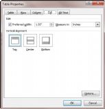
Figure 3. The Cell tab of the Table Properties dialog box.
- In the Vertical Alignment area click Center.
- Click OK.
Finally, you could create the desired lines by simply drawing the vertical lines you want. This is particularly helpful if you want the lines to be "fancy" in some way - a way that can only be achieved through using the shapes available in Word. Draw two of the same lines, place your word in a text box, adjust the lines and text box so all elements are in the desired relative positions, and then select all three items and group them. This last step is particularly important since it will ensure that the relative positions of the elements don't move around later.
PivotTables
Counting with PivotTables
Suppose you have a data table set up in Excel that represents your club membership. In the first column are the names of club members. In the second column are the cities in which the members live. If you want to find out how many people live in each city, there are several methods you can choose. One method is to create a PivotTable.
To create a PivotTable on your data, follow these steps:
- Select a cell within your data table.
- Choose the PivotTable and PivotChart Report option from the Data menu. Excel begins the PivotTable and PivotChart Wizard. (See Figure 1.)
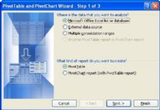
Figure 1. The PivotTable and PivotChart Wizard.
- Choose the Microsoft Excel List or Database option.
- Indicate you want to create a PivotTable, then click Next.
- In the Range box, make sure your entire data table is selected, then click Next.
- Indicate you want to put the PivotTable in a new worksheet, then click on Finish. Excel creates the bare-bones PivotTable worksheet, and the PivotTable Field List dialog box is visible.
- Drag the City field button from the PivotTable dialog box to the Row area of the PivotTable.
- Drag the Name field button from the PivotTable dialog box to the Data area of the PivotTable. Your PivotTable is complete.
The above steps won't work, however, if you are using Excel 97. Follow these steps instead:
- Select a cell within your data table.
- Choose the PivotTable Report option from the Data menu. Excel begins the PivotTable Wizard.
- Choose the Microsoft Excel List or Database option and click Next.
- In the Range box, make sure your entire data table is selected, then click Next.
- Drag the City field button to the Row area of the PivotTable builder.
- Drag the Name field button to the Data area of the PivotTable builder.
- Click on Finish. A new worksheet is created that contains your PivotTable.
Photoshop Layers tips
![]()
Converting layer styles
Converting a Layer Style to a normal pixel-based layer gives you greater control to edit the contents. To do so, add a style then right-click Effects and choose Create Layer.
View one layer
If you're working with multiple layers and you want to view one layer on its own, there's no need to hide all the others manually, simply hold down Alt and click the Eye icon of a layer to make every other layer invisible. Hold down Alt and click again to reveal them.
Invert a layer mask
After adding any Adjustment Layer, hit Cmd/Ctrl+I to invert the Layer Mask and quickly hide the effect, then paint back over the image with white to selectively reveal the adjustment.
Unlink layers and masks
You can move either a mask or an image independently of one another by clicking the link between the two thumbnails in the Layers Panel. Highlight the thumbnail you want to reposition, then grab the Move tool.
Quick copy
Hold down Alt and drag a mask, style or layer to
quickly duplicate it.
Convert the background
Double-click the Background Layer and hit OK to convert it to an editable layer.
Adjustments
Always use Adjustment Layers rather than directly editing a layer. This gives you three advantages: you can edit it at any time, control the strength with Opacity, and use a mask to make it work selectively.
Move query
When using the Move tool, right-click over a point in the image for a list of all the layers you're hovering over.
Panel Options
The Layers Panel is the most important box in Photoshop, so you'll want to make sure it's set up properly for your needs. Choose Panel Options from the Fly-out menu to select different thumbnail sizes and content.
Move layers up or down
You can move layers up or down the stack in the Layers Panel while watching the image change. Hold down Cmd/Ctrl and press ] or [. Add in Shift to move a layer right to the top or bottom.
Fill shortcuts
You can press Alt+Backspace to fill a layer or
selection with the Foreground colour, Cmd/Ctrl+Backspace to fill a layer or selection with the Background colour, or Shift+Backspace to quickly access the Fill Options.
The 50% grey layer
A new layer filled with 50% grey is useful in lots of situations. For example, you can dodge and burn with it, add texture, or manipulate a Lens Flare effect, all in a completely non-destructive way. To create a 50% grey layer, make a new layer then go to Edit>Fill, then set the Blend Mode to Overlay.
Layer group shortcut
Layer Groups are incredibly useful, but don't bother clicking on the Layer Group icon, as you'll have to add layers to the new group manually. Instead, you should highlight several layers and either drag them to this icon or alternatively hit Cmd/Ctrl+G.
Edit multiple type layers
Photoshop tips: Edit multiple type layers
To apply a change of font or size to multiple type layers at once, hold down Cmd/ Ctrl and click the layers in the Layers Panel to highlight them, then simply select the Type tool and change the settings in the Options Bar.
Layer mask views
Photoshop tips: Layer mask views
Hold down Alt and click a Layer Mask thumbnail to toggle between a view of the mask and the image. Hold down Shift and click to turn the mask on or off.
Quick full layer masks
You can Alt-click on the Layer Mask icon to add a full mask that hides everything on the layer.
Lightning fast layer copies
Hold down Cmd+Alt and drag any layer to instantly make a copy.
Colour code layers
Use colour coding to organise your Layers Panel. Right-click over a layer's eye icon to quickly access 8 colour code choices.
Select similar layers
To quickly select all layers of a similar kind, such as shape or type
layers, highlight one of them and then go to Select>Similar Layers.
Change opacity
When not using a painting tool, you can change layer Opacity
simply by pressing a number key. Hit 1 for 10%, 5 for 50%, and 0 for 100%.
Quick masking
You may be familiar with Color Range in the Select drop-down menu. But did you know that you can access a similar command through the Color Range button in the Masks Panel? (Window>Masks). This allows you to quickly make a mask by sampling colours, which can be used for making a quick spot colour effect.
Step by step: blend fire effects
A: Copy in the fire
Photoshop tips: Copy in the fire
Open a portrait image and a generic fire image, then grab the Move tool and check Auto-Select Layer and Show Transform Controls. Drag the fire image into the girl image to copy it in, then change the Blend Mode of the layer to Screen.
B: Position and warp
Photoshop tips: Position and warp
Click the bounding box to transform the fire layer, then resize, rotate and position the layer. Right-click while in Transform mode and choose Warp to wrap the fire around the body. Hit Cmd/Ctrl+J to copy the fire layer and transform again to build up the effect.
Here are five tips for Microsoft Word that are designed to be quick and efficient time-savers.
1. Quick-select sections of text
Messing around with the mouse trying to highlight exactly the section of text that you need is time-consuming and often frustrating. So here are two tips for the price of one on ways to highlight the text that you want with no fuss, no muss.
To select an entire paragraph, just make three rapid clicks anywhere on the paragraph. This will select your entire paragraph.
What if you only want to select a specific sentence instead of a whole paragraph? Well, you can do that too! On a Mac, hold down Command and click. If you`re on Windows, you`ll want to hold down Ctrl and click. The result is that you`ll select just the sentence that you`re targeting.
2. Use keyboard shortcuts for subscript and superscript
When you`re working on academic papers, you might need to frequently notate portions of text using subscript or superscript. Navigating manually to change this is a real pain, but did you know there are keyboard shortcuts to immediately put you in subscript or superscript mode? For Mac users, just hit Command plus to make text subscript. For superscript, hit Command + Shift + plus. For Windows, click Ctrl plus (for subscript) or Ctrl + Shift + plus (for superscript).
3. Instantly add a horizontal line
Have you ever wanted to put a horizontal line in your text? You don`t have to navigate to the menu bar at all to do that. In fact, all you have to do is go to a clean line, enter three hyphens in a row, and then hit enter. You`ll instantly have a horizontal line dividing your page.
4. Delete words, not individual letters
If you`ve made a wrong word choice, you don`t have to delete each character in that word individually. Instead, you can just hold down the Command key and then hit backspace (on a Mac) in order to delete the entire word that you last typed. On Windows, click Ctrl + backspace.
5. Increase or decrease font size with a keyboard shortcut
Highlight your text, and on a Mac, use Command + Shift + > to increase the font size. You can also use Command + Shift + < to decrease the font size. On Windows, use Ctrl + Shift + > or Ctrl + Shift +
Essential Photoshop shortcuts
![]()
Mastering these shortcuts will help you work smarter, save time, and graduate to true Photoshop guru level!
- Cmd/Ctrl+Shift+Alt+E will merge a copy of all Layers
- F Cycle through workspace backgrounds
- X Change your foreground and background colours
- D Reset foreground and background colours to black and white
- ] and [ Change your brush tip size
- Cmd/Ctrl+J Duplicate a layer or selection
- Space Bar Hold Space and drag to navigate around the image
- TAB Hides or shows all panels and tools
- Cmd/Ctrl+T Transform a layer
- Cmd/Ctrl+E Merge selected layer down, or merges several highlighted layers
- Cmd/Ctrl/Ctrl+Shift+Opt+S Save for web & devices
- Cmd/Ctrl+L Bring up levels box
- Cmd/Ctrl+T Open Free Transform tool
- Cmd/Ctrl+M Open Curves
- Cmd/Ctrl+B Edit Colour Balance
- Cmd/Ctrl+Shift+Opt+C Scale your image to your preferred state
- Cmd/Ctrl+Opt+G Create clipping mask
- Cmd/Ctrl+0 Fit on screen
- Cmd/Ctrl+Shift+>/< Increase/decrease size of selected text by 2pts
- Cmd/Ctrl+Option+Shift->/< Increase/decrease size of selected text by 10pts
- ]/[ Increase/decrease brush size
- Shift+F5 Fill the selection
- }/{ Increase/decrease brush hardness
- ,/. previous/next brush
- </> First/last brush
- Cmd/Ctrl+] Bring layers forward
- Cmd/Ctrl+[ Send layer back
- Cmd/Ctrl+Shift+[ Send layer to bottom of stack
- Cmd/Ctrl+Shift+] Bring layer to bottom of stack
Conditional Format that Checks for Data Type

We are trying to establish a conditional format that will alert us that text data has been entered into a cell intended for numerical data or when numerical data has been input into a cell intended for text data.
A conditional format can be used to draw attention to when an improper value (text or numeric) has been entered in a cell, but a more robust approach might be to prohibit the improper value from being entered in the first place. This can be done with the data validation capabilities of Excel.
Using data validation you can specify the type and range of data permitted in a cell, along with how stringently you want that specification followed. If you prefer to not use data validation for some reason, you can set up a conditional format that will verify if the information placed in a cell is of the data type you want. Follow these steps:
- Select the cells that you want conditionally formatted.
- With the Home tab of the ribbon displayed, click the Conditional Formatting option in the Styles group. Excel displays a palette of options related to conditional formatting.
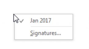
- Choose Highlight Cells Rules and then choose More Rules from the resulting submenu. Excel displays the New Formatting Rule dialog box. (See Figure 1.)
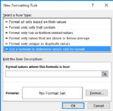
Figure 1. The New Formatting Rule dialog box.
- In the Select a Rule Type area at the top of the dialog box, choose Use a Formula to Determine Which Cells to Format.
- In the Format Values Where This Formula Is True box, enter one of the following formulas. (The first is if you want to highlight the cell if it contains text; the second if it contains a number. Make sure you replace A1 with the cell address of the cell in the upper-left corner of the range selected in step 1.)
=ISTEXT(A1)
=ISNUMBER(A1)
- Click Format to display the Format Cells dialog box.
- Using the controls in the dialog box, specify a format that you want to be used for those cells selected in step 1. For instance, you may want bold text in a red typeface.
- Click OK to dismiss the Format Cells dialog box. The formatting you specified in step 7 should now appear in the preview area for the rule.
- Click OK.
Easy Photoshop Tips
![]()
- Easier marquee selections
Hold down Alt to start a selection at the centre point with any Marquee tool, and then hold Space to temporarily move the selection around.
- Undo, undo, undo
You probably know that Cmd/Ctrl+Z is Undo, but you may not know Cmd/Ctrl+Alt+Z lets you undo more than one history state.
- 1000 history states
Go to Edit>Preferences>Performance to change the number of History states up to a maximum of 1000. Beware though of the effect that this has on performance.
- Cycle blend modes
Shift + or - will cycle through different layer Blend Modes, so long as you don't have a tool that uses Blend Mode options settings.
- Rotating patterns

You can make amazing kaleidoscopic patterns with the help of a keyboard shortcut. Cmd/Ctrl+Shift+Alt+T lets you duplicate a layer and repeat a transformation in one go. To demonstrate, we've made a narrow glowing shape by squeezing a lens flare effect, but you can use any shape, image or effect you like. First, make an initial rotation by pressing Cmd/Ctrl+T and turning slightly, then hit Enter to apply. Next, press Cmd/Ctrl+Shift+Alt+T repeatedly to create a pattern.
- Combine images with text

There's a really easy way to overlay an image on top of the text. Drop an image layer over a type layer then hold down Alt and click the line between the two layers in the Layers Panel to clip the image to the text.
- Bird's eye view
When zoomed in close, hold down H and drag in the image to instantly dart out to full screen then jump back to another area. One of the best Photoshop tips for viewing work!
- Funky backgrounds

Want to change the default grey background to something funkier? Shift€click on the background area with the Paint Bucket tool to fill it with your foreground colour. Right-click it to go back to grey.
- Close all images
To close all of your documents at the same time, Shift-click any image window's close icon.
- Spring-loaded move
While using any tool, hold Cmd/Ctrl to temporarily switch to the Move tool. Release to go back to your original tool. Note that spring-loaded keyboard shortcuts work for other tool shortcuts, too.
- Interactive zoom
For interactive zooming, hold Cmd/Ctrl+Space then drag right to zoom in, or left to zoom out. The zoom targets where your mouse icon is, so it's one of the quickest ways to navigate around an image.
- Diffuse effects
The Diffuse Glow filter can give highlights a soft ethereal feel, especially when you combine the effect with desaturation. Hit D to reset colours then go to Filter>Distort> Diffuse Glow. Keep the effect fairly subtle, then go to Image>Adjustments>Hue/ Saturation and drop the saturation down to complete the dreamlike effect.
- Step by step: select sky with channels
A: Copy Blue Channel
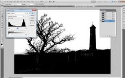
Go to Window Channel then drag the Blue Channel to the New Channel icon to duplicate it. Hit Cmd/Ctrl+L to access Levels, then drag the white and black point sliders in dramatically to make the sky totally white and the land black. Now use the Brush tool and paint with black to tidy any bits in the land.
B: Load a selection

Hold Cmd/Ctrl and click the Blue Copy Channel to load a selection of the white areas. Click back on the RGB Channel then go to the Layers Panel and add a Curves Adjustment Layer. The selection is automatically turned into a mask. Drag down on the curve to darken the sky.
So Many Signatures: An Outlook "Hack"

In the Microsoft #Outlook course, there is a lesson on "Signatures".
.png)
Signatures appear at the bottom of our Outlook messages and normally include our contact information. However, we find ourselves sending many emails that are structured very similarly to one another. We often feel like we are typing the same email over and over again, but just changing the recipient`s name or some other minor detail. To help save time (and our sanity) we can create a signature out of the body of the message. For example, maybe you need to send out a weekly reminder to your department about expense reports. And every Wednesday you find yourself typing:
"Hello Team, Please do not forget to submit last week`s expense reports by this Friday at 5 pm. Thank you."
Instead of typing it again or copying the email, create a signature that includes the previous quoted text! We can create signatures for the multiple "forms" of emails that we send out regularly which has cut down on the amount of time we spend in our Inbox.
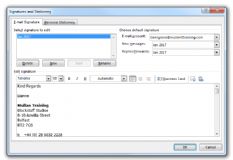
Can`t find the specific signature you saved? There is a shortcut to get to all of your signatures. You can right-click on the signature and a shortcut menu pops up.
We can also create a signature that is blank so if we are not going to include a signature in a message we can right-click and select Blank rather than selecting the signature text and deleting it.
Locked Shapes in Visio

Most shapes in Visio will allow you to resize them without a hitch. However, there are certain stencils, such as Home Plan, that come with locked shapes. If you come across a shape that will not let you resize it, don`t worry. There is a fix for that. You just need to add the Protect Shape button to your toolbar. You will find this under All Commands ...
![]()
Now to unlock the shape, you`ll follow these steps:
1. Click on the shape
2. Click the Protection button
3. Uncheck the:
- Width
- Height
.png)
You will now be able to resize the shape to your heart`s content without any other troubles!
Locked Shapes in Visio 2013
Now it`s a little different when you work in Visio 2013. What you will do in Visio 2013 to unlock a locked shape, is the following:
1. Bring up the Shape Data from the Task Panes
2. Choose Custom from the drop-down list

And that's how you fix that pesky problem of locked graphics when you are working in Visio!
Reference Shortcut

Odd Arrow Key Behaviour
If you are ever using Excel and the arrow keys don't work like you think they should, it could be because of the Scroll Lock key.
.jpg)
Normally, when you press an arrow key, Excel moves the cell highlight in the direction of the key you pressed. If the Scroll Lock key has been activated, however, Excel doesn't move the cell highlight, it instead moves the worksheet, changing what is displayed on the screen.
To solve this odd behaviour, simply press on the Scroll Lock key another time. The arrow keys should again behave as you expect them to.
Understanding the If ... End If Structure

Macros in Excel are written in a language called Visual Basic for Applications (VBA). Like any other programming language, VBA includes certain programming structures which are used to control how the program executes. One of these structures is the If ... End If structure. The most common use of this structure has the following syntax:
If condition Then
program statements
Else
program statements
End If
When a macro is executing, and this structure is encountered, Excel tests whatever condition you have defined. If the condition is true, then the program statements, the statements right after the Then keyword, are executed. If they are not true, then the statements after the Else keyword are executed. The Else keyword and any following program statements (which together make up an Else clause) are optional; you do not need to include them in your macro.

Regardless of whether the program statements in the If ... End If structure are executed, when Excel is done with the structure, the macro continues running with the statement following the End If keyword.
End-of-Month Calculations
There are many ways you can use Excel to calculate the date at the end of the next month. One such way, using the EOMONTH function. There are ways you can do it, however, without using that particular function. (Some may not want to use it because the EOMONTH function used to only be available if the Analysis Toolpak was loaded. If you couldn't count on it being loaded, it doesn't make sense to rely on the function.)
For instance, one approach is to AutoFill for the last days. Let's say you wanted the last days of a series of months in the first column, beginning at A4. All you need to do is this:
- In cell A4, enter the last day of the current month, such as 30 Apr 2017.
- In cell A5, enter the last day of next month, such as 31 May 2017.
- Select both cells, A4 and A5.
- Click on the small square handle at the bottom right corner of the selection.
- Drag the mouse downward as many cells as desired.
The result is that the area you drag over in step 5 is filled with end-of-month dates for the next however many months. Pretty cool! A slight variation on these steps could also be used:
- In cell A4, enter the last day of the current month, such as 30 Apr 2017.
- Select cell A4.
- Right-click on the small square handle at the bottom right corner of the selection.
- Drag the mouse downward as many cells as desired. When you release the mouse button, Excel displays a Context menu.
- From the Context menu, choose Fill Months.
If you are not an AutoFill type of person, and instead prefer to use formulas, you could enter the starting end-of-month date in cell A4 (it must be an actual end-of-month date) and then the following formula in A5:
=DATE(YEAR(A4),MONTH(A4)+2,1)-1
This formula calculates the date for the first day of the month two months in the future, and then subtracts one from it. The result is the last day of the next month. The formula wraps around the end of years just fine, since the DATE function increments the years properly if the month value provided is greater than 12.
Another formulaic approach is to use the following:
=A4+32-DAY(A4+32)
This formula works because it adds 32 to the starting date (to make sure you are past the end of the following month), and then subtracts the number of days the result is past the end of the month.
Making Pane Settings Persist
If we freeze panes in a worksheet and then save the workbook, the next time we open that workbook the previously frozen panes no longer appear. Each time we open the workbook, we need to reset the panes. We don't think it used to be this way in older versions of Excel and wonder if there is some setting we need to make or wonder, perhaps, if Excel has changed how it handles panes. We want to save the pane settings with the workbook so they persist from one usage to another.
The default behavior of the latest versions of Excel is that your pane settings should be persistent, just as we remember in older versions of Excel. If that is apparently not happening for you, there are a few things you can check:
- See if someone else is updating or using the workbook and, while doing so, removing the panes.
- Check to see if the workbook has a macro that runs automatically when starting that removes the panes. You might try looking for the text "Freeze Panes" in the macros.)
- See if the workbook is actually being saved in a non-Excel format, such as CSV or HTML. Other formats don't necessarily hold on to some settings, such as panes. (Save the file in XLS or XLSM format to see if that fixes the problem.)
- Is the workbook, when open, being worked with using multiple windows? If so, and one of the windows doesn't use panes, the settings in the last-closed window are those that will "stick" in the workbook.
- Check if the workbook is being shared with others. Some users report an oddity where pane settings may not save properly in shared workbooks.
- Are filters being used in the workbook? If you apply filters, then set panes, and finally remove filters, the panes may also go away.
If none of those ring a bell with you, try starting with a brand new, blank workbook. Put some test data in it, freeze the panes, and then save it. Exit Excel and open the workbook again. If the panes are still there, then this is a good sign that the problem is with the other workbook only. In that case, it could be that the workbook is becoming corrupted (for some reason) and you may need to work on getting your data into a different workbook.
There are two other things you can do, if you desire. One is to simply save a custom view of your worksheet, with the panes in place. You should then be able to load the custom view at a later time and have the pane settings be present (along with many other settings) so that you can continue working with the workbook.
The other thing you could try is to create your own macro that sets the panes as you want them to appear. Here's an example:
Private Sub Workbook_Open()
Sheets("Sheet1").Range("D4").Select
ActiveWindow.FreezePanes = True
End Sub
This macro would be added to the Workbook module, and you'll need to change the cell reference (D4) and worksheet name (Sheet1) to reflect where you want the panes set. You could also, if desired, change the code to a "regular" macro that could be assigned to a shortcut key or the Quick Access Toolbar. That way you could use the macro to set similar panes in any worksheet, with the click of a button.
Sub SetPanes()
ActiveSheet.Range("D4").Select
ActiveWindow.FreezePanes = True
End Sub
Using Stored Views
Once you have defined the views for a worksheet, you can use them to look at your information in different ways quickly. To select different views, follow these steps:
1. Display the View tab of the ribbon.
2. Click the Custom Views tool in the Workbook Views group. Excel displays the Custom Views dialog box. (See Figure 1.)
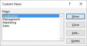
Figure 1. The Custom Views dialog box.
3. Select a view from those listed in the dialog box.
4. Click on the Show button. Your display settings are changed to reflect what was previously saved in the view.
Formatting Currency
There is a way to easily format cells so what would normally appear as $10,000.00 would appear as $10.000,00. This format being described is the difference between the US method of displaying figures (using commas as thousand separators and a period as a decimal sign) and the European method of displaying figures (using periods as thousand separators and a comma as a decimal sign).
There are three ways you can accomplish a switch. The easiest method is to simply change the Regional Settings in Windows. The exact way you do this depends on the version of Windows you are using, but in general there is a choice in the Windows Control Panel that allows you to specify regional settings. All you need to do is modify those settings to match the numeric display format desired. The change will affect not only the display of numbers in Excel, but in other Windows-compliant programs, as well.
The second method is to use a formula to handle the numeric display. This has the drawback of converting the numeric value to text, but it could be easily done. For instance, let's assume that you have the formatted numeric value $10,000.00 in cell A1. The following formula, in a different cell, would display the text $10.000,00:
=SUBSTITUTE(SUBSTITUTE(SUBSTITUTE(TEXT(A1,
"$#,##0.00"),".","^"),",","."),"^",",")
This formula first converts the number to an initial currency format in text. Then the SUBSTITUTE function is used to first change "." to "^" ("^" is used as a temporary placeholder), and then change "," to ".", and finally "^" to ",".
The final method has the advantage of leaving your numbers as numbers, instead relying on a custom format. All you need to do is to multiply your values by 100 and then use the following custom format:
#"."###"."###","##
The format allows any number up to 9.999.999,00 to be used. If you deal with numbers that have more than two decimal places, you will need to adjust your custom format accordingly, or adjust the value being displayed so that it has nothing to the right of the decimal point after it is multiplied by 100.
Summing Based on Part of the Information in a Cell
We have a worksheet that includes information for all the parts in our warehouse. In this sheet, part numbers are shown in column A using the format 12345 XXX, where XXX represents a location code. This means we could have multiple entries on the worksheet for the same part numbers, but each entry representing a different location for that part. We need a formula that sums the values associated with each part number, regardless of its location code. Thus, we need a way to sum the quantity column related to parts 12345 ABC, 12345 DEF, 12345 GHI, etc. We need a way to do this without splitting the location code to a different column.
There is more than one way to get the desired answer. For the sake of the examples in this tip, assume that the part numbers are in column A and that the quantities for each part are in column B. It is these quantities that need to be summed, based upon just a portion of what is in each cell in column A. Further, you can put the part number (minus the location code) desired in cell D2.
The first potential solution is to use the SUMPRODUCT function, in this manner:
=SUMPRODUCT((VALUE(LEFT(A2:A49,FIND(" ",A2:A49)))=D2),B2:B49)
This formula checks the values in the range A2:A49. You should make sure that this range reflects the range of your actual data. If you generalize the formula so that it looks at all of columns A and B (as in A:A and B:B), you'll get a #VALUE error, since it tries to apply the formula to empty cells in the columns.
You can get a similar result by using an array formula such as this:
=SUM(B:B*(LEFT(A2:A49,5)=TEXT(D2,"@")))
Remember, again, that this is an array formula, so you need to enter it by pressing Shift+Ctrl+Enter. Note, as well, that this formula converts the value in D2 to text for the comparison. This wasn't done in the previous formula because there the substring picked out of column A was converted to a numeric value using the VALUE function.
You can also use the DSUM function to construct a working formula. Let's assume that the part numbers (column A) have a column header in cell A1. Copy this column header (such as "Part Num") to another cell in the worksheet, such as cell D1. In cell D2, enter the part number, without its location code, followed by an asterisk. For example, you could enter "12345*" (without the quote marks) into cell D2. With that specification set up, you can then use this formula:
=DSUM($A$1:$B$49,$B$1,D1:D2)
This formula uses the specification in cell D2 (the characters 12345 followed by anything) as a key to which values from column B should be summed.
Finally, if you had the same specification in cell D2 as you used with the DSUM approach, you could use a very simple SUMIF function, in this manner:
=SUMIF(A:A,D2,B:B)
Note that this approach allows you to use the full column ranges (A:A and B:B) in the formula.
If your part numbers (in column A) are not as consistent in their format as you might like, then you may be better creating a user-defined function to find your quantities. For instance, if your part numbers aren't always the same length or if the part numbers can contain both digits and letters or dashes, then a UDF is the way to go. The following example works great; it keys on the presence of at least one space in the value. (Kathy indicated that a space separated the part number from the location code.)
Function AddPrtQty(ByVal Parts As Range, PartsQty As Range, _
FindPart As Variant) As Long
Dim Pos As Integer
Dim Pos2 As Integer
Dim i As Long
Dim tmp As String
Dim tmpSum As Long
Dim PC As Long
PC = Parts.Count
If PartsQty.Count <> PC Then
MsgBox "Parts and PartsQty must be the same length", vbCritical
Exit Function
End If
For i = 1 To PC
Pos = InStr(1, Parts(i), " ")
Pos2 = InStr(Pos + 1, Parts(i), " ")
If Pos2 > Pos And Len(Parts(i)) > Pos + 1 Then
tmp = CStr(Trim(Left(Parts(i), Pos2 - 1)))
ElseIf Pos > 0 And Len(Parts(i)) > 0 Then
tmp = CStr(Trim(Left(Parts(i), Pos - 1)))
End If
If CStr(Trim(tmp)) = CStr(Trim(FindPart)) Then
tmpSum = tmpSum + PartStock(i)
End If
Next i
AddPrtQty = tmpSum
End Function
To use the function, in your worksheet call it using two ranges and the part number you want:
=AddPrtQty(A2:A49,B2:B49,"GB7-QWY2")
Picking a Group of Cells
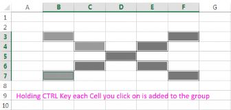
Excel allows you to define a group of cells in preparation for doing an action, such as formatting the cells. This is different than picking a range of cells, however. A range of cells is contiguous in nature - every cell between a starting and ending point is selected. A group of cells does not need to be contiguous. Instead, they can be anywhere on the worksheet.

To put together your own group of cells, you need to use the mouse. Click on the first cell in the group. As you click on each subsequent cell in the group, simply hold down the Ctrl key. Each cell you click on is added to the group. If you click on a cell a second time (with the Ctrl key pressed), the cell is removed from the group. If you click on any cell without holding down the Ctrl key, that cell is selected and the selection set is gone.
Deleting Rows before a Cutoff Date
We have a large worksheet containing several thousand rows of data. Column B contains a date, and we need to delete all the rows in which the date in column B is earlier than a specific cut-off date. We wonder about the easiest way to do this for so much data.
This is rather easy to do, with the approach you use dependent on how often you need to do it and how you want to work with your data. If you don't care what order your data is in, then the easiest method is what I refer to as the "sort and delete" method:
- Select cell B2. (This assumes that B2 is the first date in your rows of data because row 1 contains headers.)
- Display the Data tab of the ribbon.
- Click the Sort Oldest to Newest tool. Excel sorts the data according to the dates in column B, with the oldest date in row 2.
- Select and delete the rows that contain dates before your cut-off.
This works great if you only need to perform that task once in a while and if you don't mind the rows in the data being reordered. If reordering is a problem, then you may want to add a column to your data and fill that column with values from 1 to however many rows of data you have. You can then perform the "sort and delete" method, but afterwards resort your data based on the values in the column you added.
Of course, you could also use a "filter and delete" method, which will leave your data in its original order without the need of a helper column:
- Select cell B2. (This assumes that B2 is the first date in your rows of data because row 1 contains headers.)
- Press Ctrl+Shift+L. Excel applies AutoFilter to your data. (You should be able to see the small drop-down arrows next to the headers in row 1.)
- Click the drop-down arrow next to the Date header in cell B1. Excel displays some sorting and filtering options.
- Hover your mouse pointer over the Date Filters option. Excel displays even more options.
- Choose the Before option. Excel displays the Custom AutoFilter dialog box.
- In the box to the right of "Is Before," specify a date one day after your cut-off date.
- Click OK. Excel applies the filter and you can only see those rows that are at or before your cut-off date.
- Select all the rows, but not row 1. (That's because row 1 contains your headers.)
- Display the Home tab of the ribbon.
- Click the Delete tool. Excel deletes all the selected rows.
- Display the Data tab of the ribbon.
- Click the Filter tool to remove the AutoFilter.
If you need to perform the task of removing rows often, then you won't be able to beat the convenience of using a macro. The following macro assumes that you've placed the cut-off date into cell K1. It grabs this date and then looks at each row in your data, deleting any rows that are before this cut-off date.
Sub DeleteRowsBeforeCutoff()
Dim LastRow As Integer
Dim J As Integer
Application.ScreenUpdating = False
LastRow = Cells(Rows.Count, 2).End(xlUp).Row
For J = LastRow To 1 Step -1
If Cells(J, 2) < [K1] Then
Cells(J, 2).EntireRow.Delete
End If
Next J
Application.ScreenUpdating = True
End Sub
Correlation Analysis
Web data analysis comes with its own set of data inconsistencies and irregularities that cannot be explained by simple math. Sometimes you may notice that your website bounce rate changes with the day of the week, and sometimes the conversion rate will change with traffic. This happens when one data set (visits) shares positive or negative relationship with another data set (conversion).
Pearson`s correlation is the best way to measure the positive and the negative correlation of data to rule out the data inconsistencies and establish a baseline.
MS Excel 2007 is equipped with Correlation function and can be used to perform a quick analysis.
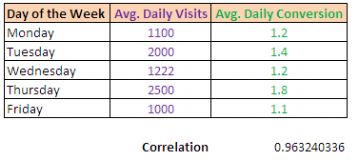
Let`s assume that we want to see the relationship between the daily visits and the website conversion.
a. Enter the visit and the conversion data on the Excel spreadsheet.
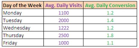
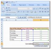
b. Place the cursor on any empty cell in the spreadsheet. This cell will be used to display the Pearson`s correlation coefficient. Press F2 to enter the formula for correlation and type "=Correl" and hit Tab key.
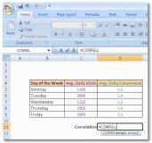
c. Once you hit the Tab key, the cursor will be placed in the bracket, and you will be allowed to select the array data. Select your first data column (avg. daily visits) for the array1 and second data column (avg. daily conversion) for the array2. Close the bracket and then hit the Enter key.
d. The value displayed in the cell (0.963240336) will be the correlation between the avg. daily visits and avg. daily conversion. In this case, the daily visits show a high positive correlation with conversion (greater than zero is positive and less than zero is negative. Zero is no correlation).
Word - How to Save Images from MS Word Document
- If you want to save one or few pictures from an MS Word document, you can take right click on the image and select ''Save as Picture...'' option. This feature has been made available in the recent versions of MS Word. But what if you have 200 images in the document?
- The quickest and easiest method of saving all the images from a Word document is to save the document as a webpage. If you know HTML programming, you would understand that a webpage refers to resources like images stored as individual files.
So, when we save a Word document as webpage, MS Word document becomes an HTML page and all the embedded images get stored in a separate folder. We can use this operation to get images out of the Word document.
- Open the MS Word document containing images
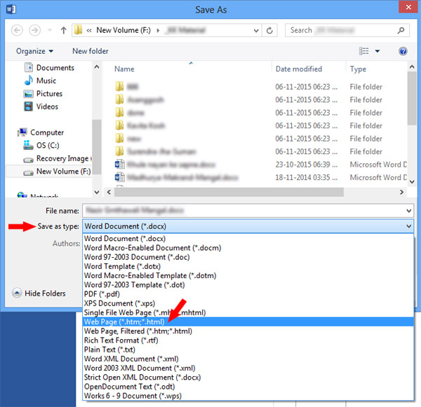
- Go to File ans then select Save As
- Save As dialog box will appear
- Select Web Page from Save as type list
- Click Save button to save the document as a webpage
- Open Windows Explorer and browse to the location where you have saved the document as webpage
- In this location, you will find a newly created folder with the same name as that of the MS Word document. This folder will contain all the images that were there in the document. There might be some other files as well, but you can ignore them
- You have got the images as files. Now you can use or edit them separately
Converting Numeric Values to Times
We have a lot of worksheets that contain times. The problem is that the times are in the format "1300" instead of the format "13:00." Thus, Excel sees them as regular numeric values instead of recognizing them as times. Sam wants them to be converted to actual time values.
There are several ways you can approach this task. One way is to use the TIME function to convert the value to a time, as shown here:
=TIME(LEFT(A1,2),RIGHT(A1,2),)
This formula assumes that the time in cell A1 will always contain four digits. If it does not (for instance, it might be 427 instead of 0427), then the formula needs to be modified slightly:
=TIME(LEFT(A1,LEN(A1)-2),RIGHT(A1,2),)
The formula basically pulls the leftmost digit (or digits) and uses them for the hours argument of the TIME function, and then uses the two rightmost digits for the minutes argument. TIME returns an actual time value, formatted as such in the cell.
A similar formulaic approach can be taken using the TIMEVALUE function:
=TIMEVALUE(REPLACE(A1,LEN(A1)-1,0,":"))
This formula uses REPLACE to insert a colon in the proper place, and then TIMEVALUE converts the result into a time value. You will need to format the resulting cell so that it displays the time as you want.
Another variation on the formulaic approach is to use the TEXT function, in this manner:
=TEXT(A1,"00\:00")
This returns an actual time value, which you will then need to format properly to be displayed as a time.
Another approach is to simply do the math on the original time to convert it to a time value used by Excel. This is easy once you realize that time values are nothing more than a fractional part of a day. Thus, a time value is a number between 0 and 1, derived by dividing the hours by 24 (the hours in a day) and the minutes by 1440 (the minutes in a day). Here is a formula that does that:
=INT(A1/100)/24+MOD(A1,100)/1440
This determines the hour portion of the original value, which is then divided by 24. The minute portion (the part left over from the original value) is then divided by 1440 and added to the first part. You can then format the result as a time, and it works perfectly.
All of the formulas described so far utilize a new column in order to do the conversions. This is handy, but you may want to actually convert the value in-place, without the need for a formula. This is where a macro can come in handy. The following macro will convert whatever cells you have selected into time values and format the cells appropriately:
Sub NumberToTime()
Dim rCell As Range
Dim iHours As Integer
Dim iMins As Integer
For Each rCell In Selection
If IsNumeric(rCell.Value) And Len(rCell.Value) > 0 Then
iHours = rCell.Value \ 100
iMins = rCell.Value Mod 100
rCell.Value = (iHours + iMins / 60) / 24
rCell.NumberFormat = "h:mm AM/PM"
End If
Next
End Sub
The macro uses an integer division to determine the number of hours (iHours) and stuffs the remainder into iMins. This is then adjusted into a time value and placed back into the cell, which is then formatted as a time. You can change the cell format, if desired, to any of the other time formats supported by Excel.
Incrementing Numeric Portions of Serial Numbers
If you have a range of serial numbers in the format A12345678B and you would like to find a formula that will increment the numeric portion of the serial numbers by 1. Thus, the next number in sequence would be A12345679B, then A12345680B.
There are actually a couple of ways you can go about this, and the first doesn't really involve a formula at all. Instead, you can create a custom format that displays your serial number; the format should look like this:
"A"#"B"
Then, in a cell that has this format applied, you only need to include the numeric portion of the serial number (12345678). You can then use regular AutoFill techniques to fill out as many cells as necessary with the serial number.
If you really want to use a formula, then the following should work just fine as long as the pattern for the serial number is a single letter, eight numeric digits, and a single terminating letter:
=LEFT(A1,1) & MID(A1,2,8)+1 & RIGHT(A1,1)
This assumes that cell A1 contains the beginning serial number. If you put the formula in cell A2, it could be copied down as many times as necessary for the desired number of serial numbers.
If the numeric portion of the serial number could start with leading zeroes, then you need to use a different formula to provide the proper zero padding:
=LEFT(A1,1) & TEXT(VALUE(MID(A1,2,8))+1,"00000000") & RIGHT(A1,1)
Excel - Limiting Input by Time of Day
There are two general ways you can go about this. One approach is to use Data Validation to check the time and either allow or disallow data entry.
- Select all the cells in the worksheet.
- Display the Data tab of the ribbon.
- Click the Data Validation tool in the Data Tools group. Excel displays the Data Validation dialog box. (See Figure 1.)
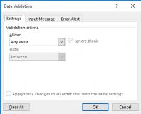
- Using the Allow drop-down list, choose Custom.
- Enter the following in the Formula box:
=OR(24*MOD(NOW(),1)18.5)
- Make changes on the Error Alert tab, as desired.
- Click OK.
The problem with this approach is in the very first step: You need to select all the cells in the worksheet in order to prevent data being entered in any of them. Plus, if you already are using Data Validation in any of the cells, this approach will overwrite those settings.
For these reasons, it may be better to use a macro-based approach. All such approaches can utilize event handlers to check for any changes. The following relies on the Worksheet_Change event, which means it is triggered only when Excel detects a change in the worksheet.
Private Sub Worksheet_Change(ByVal Target As Range)
Dim sMsg As String
sMsg = "No entries allowed between 4:00 pm and 6:30 pm!"
If Time >= "4:00:00 PM" And Time
MsgBox sMsg, vbCritical
With Application
.EnableEvents = False
.Undo ' This undoes the change the person made
.EnableEvents = True
End With
End If
End Sub
Essentially, every time there is a change in the worksheet, the handler checks to see if it is between 4:00 pm and 6:30 pm. If it is, then a message box is displayed to indicate the error, and then the .Undo method is used to roll back any change that was attempted.
If you prefer, you could take a different approach and protect the worksheet if it is within the banned time:
Private Sub Worksheet_Activate()
If Time >= "4:00:00 PM" And Time
ActiveSheet.Protect
MsgBox "Worksheet is protected."
Else
ActiveSheet.Unprotect
MsgBox "You are free to edit now."
End If
End Sub
The Worksheet_Activate event handler is invoked every time the worksheet is activated (selected). If the worksheet is activated anytime outside of the banned time, then it is unprotected. Of course, the user could still manually unprotect the worksheet even during the banned time, so it is a good idea to use this approach in conjunction with an approach that is triggered every time a change is attempted, as discuss Excel includes several different form controls that you can add to your worksheets. One of ted earlier.
Excel - Adding and Using a Combo Box
Excel includes several different form controls that you can add to your worksheets. One of these controls is a combo box. This control allows you to pick an option from a drop-down list, and then determine what was picked. To create a combo box, follow these steps:
Somewhere in your worksheet, create a list that specifies what you want to appear in the combo box. For instance, if you have a list of names you want to appear in the combo box, create that list of names in your worksheet. (For this example, let's assume that you create the list in cells K7 through K13.)
- Make sure the Forms toolbar is displayed. (Choose View | Toolbars | Forms.)
- Click on the Combo Box tool in the toolbar. The mouse pointer changes to a small crosshair.
- Create the actual combo box by clicking and dragging to define the parameters of the control. When you release the mouse button, the combo box appears in your worksheet.
- Right-click on the newly created combo box. A Context menu appears.
- Choose the Format Control option from the Context menu. Excel displays the Control tab of the Format Control dialog box.(See Figure 1.)
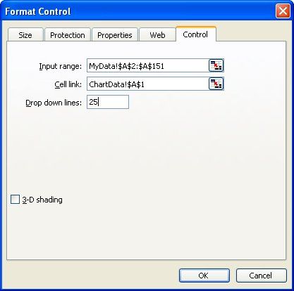
- In the Input Range box, specify the range used by the list you created in step 1. (For instance, K7:K13.) You can also click once in the Input Range box and then use the mouse to select the range in the worksheet.
- In the Cell Link box, specify the worksheet cell that you want to contain the index value of what is selected in the combo box.
- Click on OK.
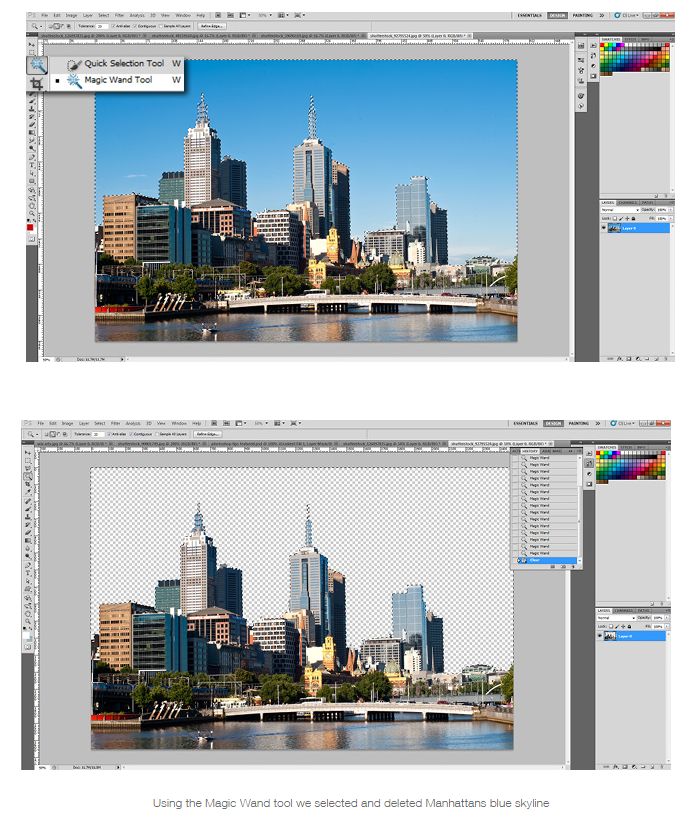
Photoshop Magic Wand Tool
The Magic Wand is another selection tool, ideal for when you are working with a background that is very monotone and consistent. If you have a clearly defined color that you want to choose in an image, this is the tool for you. For example, the Magic Wand is great when you want to select a white background or a clear blue sky.
Choose the magic wand tool from the tools panel and click on the part of the image you want to select. Make sure that you toggled the ''add to selection'' option on the top bar (icon of two squares) so you can keep on adding colors and tones to your selection.
Excel Function Keys and Shortcuts

Function Keys in Excel are a handy and faster way of doing certain tasks by using keyboard instead of mouse. Function keys provide same output in all versions of Excel making it easier to recall.
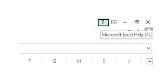
F1 Key:
''F1'' is used for opening ''Excel Help''. Its output is same as obtained by clicking on ''question mark button'' available on top right hand side of your excel sheets as highlighted in below image.
Alt + F1:
If you use ''Alt and F1'' Keys together then it will insert a new chart in your excel and will open the chart options. It is a column chart by default as shown in below image.

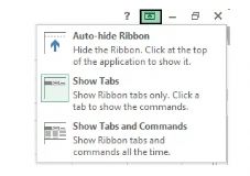
Ctrl + F1:
You can minimize or maximize the ribbon of excel by pressing ''Ctrl & F1'' Keys together. By minimizing the ribbon only tab names will be displayed on the ribbon. This could also be achieved by clicking on the button highlighted in below image:
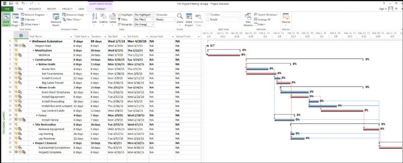
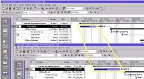
Estimate time needed and actual time used

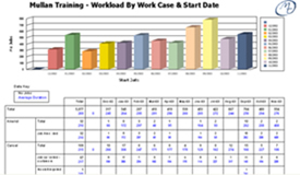
The application's Gantt chart has a bar for each task representing the time at which the task will be done and how long it will take. If you grab the left edge of a bar and drag, you can indicate how far along you are. If you run into problems (gee, that never happens) and the task is going to take longer,you can grab the right edge and extend the time needed (see the picture below).
Mullan Training will be providing regular Tips and Tricks to help enhance your use of Microsoft Excel, Word and other applications.
Keep up to date with these tips by liking our Facebook page!
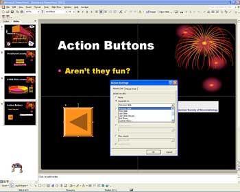
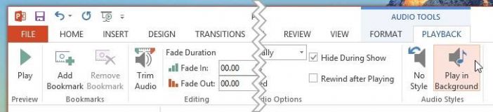
Play Music in the Background During PowerPoint Presentations
Here's a fun tip: punch up your PowerPoint presentation with some tunes. While playing music in the background certainly isn't always appropriate, adding audio for the duration of your presentation is an easy process that can make your slides a bit more interesting.
First, you'll want to ensure that you have your music or audio file saved on your computer (or an accessible cloud location) and that you have the rights to play the music in the setting where you're presenting. See this page for audio formats that PowerPoint can use. Then:
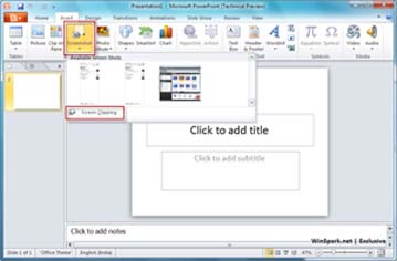
- From the Insert tab, select the Audio button.
- Locate the music file you wish to include and click Insert.
- From the Playback tab, click Play in Background.
If your presentation will be longer than the song you chose, you can add more than one song. Simply repeat steps 1-3 on any slide on which you want to add a new or additional track.
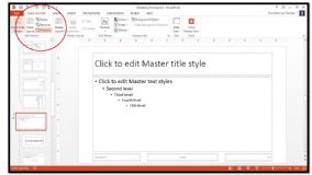
Be the Boss of Your Slides by Using the Slide Master in PowerPoint
You've finally finished the first slide in your PowerPoint presentation. The formatting, colors, and transitions are, in a word, perfection... and now you only have 27 slides to go.
Never fear! With PowerPoint 2013/2016, there's no need to waste time duplicating your formatting for each additional slide in your presentation. Once you get a slide exactly the way you want it, the Slide Master allows you to consistently format every slide, all at once, all in one place, and with one simple step. You'll be able to spend more time focusing on the content of your presentation, rather than its formatting.
To quickly format all of the slides in a presentation in PowerPoint 2013/2016:
- Open the View tab and select Slide Master.
- In the Slide Master View, the Master Slide and all the slide layouts in the theme are shown.
- Click on the Master Slide (or the slide you want to adjust) and edit it how you want.
- The changes will translate to each of the slides in the theme.
- You can see how your changes impact each slide layout so you can edit your design till you get it right.
- When you go back to Normal View, your changes will be saved.
How to Import/Migrate Gmail Contacts to Outlook
If you use Outlook 2013 or the Outlook Web App, it's easy to import contacts from other email services. If you've moved from Google Apps to Office 365, from Google Apps for Work to Office 365 for Business, or you're just using both email clients and want to have the same contacts in both, you can follow the instructions below.
To export Gmail contacts:
- From your Gmail account, click Gmail -> Contacts.
- Click More >.
- Click Export.
- Select the contact group you wish to export.
- Select the export format Outlook CSV format (for importing into Outlook or another application).
- Click Export.
- When prompted, click Save as, and browse to a location to save the file.
To import from Outlook 2013:
- From the FILEtab, select Open & Export.
- Select Import/Export.
- In the Import and Export Wizard, select Import from another program or file.
- Click Next.
- Select Comma Separated Values.
- Click Next.
- In the Import a File box, browse to and select the .csv file you saved your Gmail contacts to.
- Select Replace duplicates with items imported, Allow duplicates to be created, or Do not import duplicate items.
- Click Next.
- In the folder list, select the contacts folder where you want to import your contacts to, and click Next.
- Click Finish.
To import from Outlook Web App:
- Select People from the app launcher.
- Select the settings gear, then click Options.
- Select Import contacts under People.
- Click Browse and select the .csv file you saved your Gmail contacts to.
- Click Import.
These 4 Keyboard Shortcuts in PowerPoint Will Make Presentations a Breeze
Beginning to build a presentation PowerPoint can be quite a journey and an undertaking. To make it easier along the way, use these four shortcuts to move swiftly while you create your masterpiece.
Increase or Decrease Font Size
To quickly increase or decrease your font in PowerPoint, select the font you want to adjust and hit CTRL + Shift + < or >.
Make it Simple
When you are playing around with the text formatting, this keyboard is great to clear your slate. Press CTRL and the spacebar to remove all formatting.
Create a New Slide Within Your Presentation
Use CTRL + M to create a new slide. Don't get confused with CTRL + N, this will open up a new PowerPoint presentation.
Tab Around All Objects on Your Slide
Objects can add up in PowerPoint. To quickly move between them instead of carefully selecting the one you want and having to click over and over again, use Shift+Tab to move through them.
How to Customize the Quick Access Toolbar in Office 2013

Today we're going to look at an often-overlooked secret weapon for productivity in Office 2013: the Quick Access Toolbar. Customizing this toolbar is one of the best ways to save time by creating shortcuts to your frequently-used commands in each Office product.
What is the Quick Access Toolbar?
You'll see the Quick Access Toolbar above the Ribbon (by default) on Office 2013 programs like Excel, Word, PowerPoint, and Outlook. It's the home for one-click icons for your favorite or most often used commands and actions.
For example, if you frequently freeze panes in Excel, you can add that command to the Quick Access Toolbar so you can access it with a single click, rather than navigating to the View tab first.
How do you customize the Quick Access Toolbar?
If you want to add a command from the Ribbon, all you have to do is right-click and select Add to Quick Access Toolbar.
If you want to add a command that you can't right-click, open the drop-down menu in the toolbar and select More Commands. From there, you can choose an action from the Popular Commands section, or select and choose from another option, like All Commands, in the drop-down menu.
Once you have your Quick Access Toolbar customized to your liking, you can get used to using those icons to take actions rather than navigating through the Ribbon. You also may wish to hide the Ribbon to save space and simplify your screen.
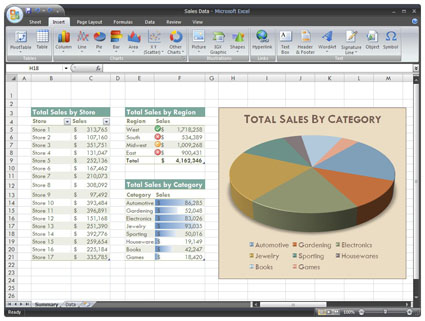
Easily Embed an Excel Spreadsheet in OneNote

OneNote allows you two kinds of information into notebooks, including other Office files. Adding an Excel spreadsheet to your OneNote page is a great way to create a copy of your Excel data to view in OneNote, so you don't have to switch back and forth between applications.
There are a few different ways to embed your spreadsheet. Begin from the Insert tab in OneNote:
- To insert a blank spreadsheet, select Table -> New Excel Spreadsheet or Spreadsheet -> New Excel Spreadsheet
- To insert an existing spreadsheet, select Spreadsheet -> Existing Excel Spreadsheet.
Note This process is best done when you don't have further changes to make to your Excel spreadsheet. Changes made in OneNote won't appear in the original Excel file, and vice versa-changes made in the Excel file won't appear on the OneNote page.
Pop-Up Comments for Graphics
We know how to add comments to cells so that when you hover the mouse over the cell you can see the comment. We would like to do the same thing with graphics - have a comment or pop-up box appear when a person hovers the mouse over a graphic placed in a worksheet. While we could adjust cell size to match the graphics and then attach the comment to the cell, the size of the graphics we are using really doesn't make that practical. We wonder if there is a way to have pop-up comments appear when someone moves the mouse over a graphic in a worksheet.
There is no way to do this using the Comments feature of Excel, but there are some workarounds. The first involves using hyperlinks. Just follow these steps:
1. Insert the graphic in your worksheet and size as desired.
2. Select the graphic (click on it once).
3. Press Ctrl+K. Excel displays the Insert Hyperlink dialog box. (See Figure 1.)
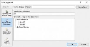
Figure 1. The Insert Hyperlink dialog box.
4. Click the Place In This Document button.
5 If desired, in the Type the Cell Reference box, enter the address of a cell close to or behind your graphic.
6. Click the ScreenTip button. Excel displays the Set Hyperlink ScreenTip dialog box.
7. Enter the text you want to be displayed.
8. Click on OK to dismiss the Hyperlink ScreenTip dialog box.
9. Click on the OK button to dismiss the Insert Hyperlink dialog box.
The result is that when someone hovers the mouse pointer over the graphic, a small note appears - usually below the graphic - that contains the ScreenTip text. It isn't quite as noticeable as a regular Excel Comment, but it does provide a little assistance.
If you want something a bit harder to miss, then a macro might be helpful. There are a number of different ways you could approach a macro-based solution, but perhaps the easiest is to simply create a macro such as the following:
Sub MyMacro()
MsgBox "This is my comment"
End Sub
Back in your worksheet, right-click on the graphics and choose Assign Macro from the resulting Context menu. Excel shows you a list of all the macros available to you; you should pick the short one you just created (in the example above it is "MyMacro").
Now, when you click on the graphic, you see a message box that contains whatever text you specified in your macro. It isn't quite as automatic as only requiring the person to scroll over the graphic, but it does provide a handy way to convey a lot of information to the user.
Setting Up Custom Auto Filtering
When we are using Excel's Auto Filtering feature, we may want to display information in our list according to a custom set of criteria.
Excel makes this easy to do. All we need to do is the following:
1. If Auto Filtering is not already turned on, display the Data tab of the ribbon and click the Filter tool.
2. Use the drop-down arrow to the right of a column label to select Number Filters | Custom Filter or Text Filters | Custom Filter. (The names of the options, and thus the choices you make, depend on the composition of your data.) Excel displays the Custom AutoFilter dialog box. (See Figure 1.)
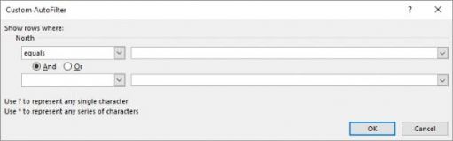
Figure 1. The Custom AutoFilter dialog box.
3. Use the controls in the dialog box to set the criteria you want to be used for filtering your list.
4. Click on OK.
We can use the Custom AutoFilter dialog box to set any combination of criteria that we need. For instance, we can indicate that we want to see any values below, within, or above any given thresholds we desire. The filtering criteria will even work just fine with text values. For instance, we can cause Excel to display only records that are greater than AE. This means that anything beginning with AA through AE won't be displayed in the filtered list.
We should note that Excel also provides wildcard characters we can use to filter text values. These are the same wildcards we can use in specifying file names at the Windows command prompt. For instance, the question mark matches any single character, and the asterisk matches any number of characters. Thus, if we wanted to only display records that have the letter T in the third character position, we would use the equal sign operator (=) and a value of ??T*. This means the first two characters can be anything, the third character must be a T, and the rest can be anything.
-
3/3/2025
Intro to Microsoft PowerPoint Training from Belfast Northern Ireland - Online Training Course -
31/3/2025
Microsoft 365 training courses in Word, Excel, Access, Outlook, Powerpoint, Sharepoint in Belfast and Omagh Northern Ireland -
26/3/2025
Microsoft Sharepoint Introduction Training Course in Belfast NI -
3/3/2025
Data Visualisation & Presentation Techniques with Mullan IT Training -
3/3/2025
CITB - The Construction Industry Training Board have included Mullan Training on their Approved List We deliver Trainings in Belfast Northern Ireland OR On Customer's Own Premises -
3/3/2025
IT/Computer Room Hire in Belfast City Centre (Opposite Europa Hotel) - Call now to book -
3/3/2025
Microsoft 365 Training Courses now available inc Belfast, Omagh, Derry, Newry and Throughout Northern Ireland -
30/4/2025
Microsoft Visio Training from Belfast Northern Ireland - Maximise the potential of the Visio application -
20/3/2025
1 day Adv Microsoft Excel CourseTraining in Belfast Northern Ireland OR On your Own Premises - Places Available - Call Now to Book -
6/5/2025
Intro to Crystal Reports Training from Belfast Northern Ireland - Virtual, Online - Learn how to create powerful and dynamic reports, presenting your data in an attractive format -
3/3/2025
Hot Course - 2 Day Advanced Microsoft Excel Course Training - CALL NOW TO BOOK -
14/4/2025
CLASSROOM & ONLINE Power BI Level 1 course -
3/3/2025
HOT COURSE - Intro to Microsoft Visio Training in Belfast Northern Ireland OR Virtually - CALL NOW to secure a place on this course -
3/3/2025
Need to Produce and Deliver Professional Presentations? Book NOW on our Advanced Microsoft PowerPoint course Training in Belfast Northern Ireland OR On your Own Premises - Limited places available -
25/3/2025
Introduction to Microsoft Project Training from Belfast Northern Ireland - Classroom Based Training & Via Our Online Classrooms -
17/4/2025
HOT COURSE - Introduction to Microsoft Excel Training in Belfast Northern Ireland OR On your Own Premises - Call NOW to Book -
14/4/2025
New Course - Microsoft Power BI Introduction training from Belfast Northern Ireland - Classroom & Online Training -
3/3/2025
Power BI Paginated Report Builder